신경망 모델의 필요성에 대해 언급하고 그 예시를 들어 같이 설명을 하겠습니다.
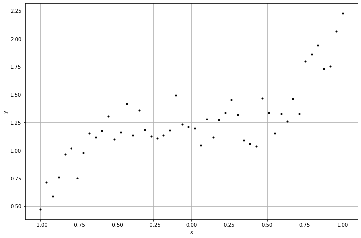
이 그래프를 보았을 때, 바로 방정식을 작성할 수 있을까요?
아마 수학을 많이 공부하신 분이라면 3차방정식이라 생각할 것입니다. 물론 이렇게 단순한 그래프라면 사람이 눈으로 보고 찾을 수도 있습니다. 하지만 우리가 사용하는 데이터는 항상 평면에만 있는 것이 아닌, 다차원의 공간 상에 있게 됩니다. 그럴 때는 직접 찾는 것이 아니라 컴퓨터의 힘을 빌려 알아내야 합니다.
#특성값과 레이블
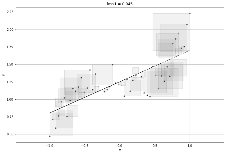
features1 = np.array([[xval] for xval in x_train])
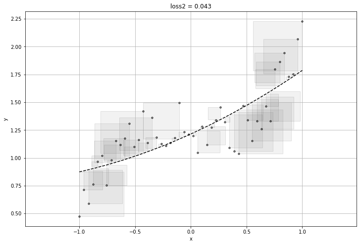
features2 = np.array([[xval**2, xval] for xval in x_train])
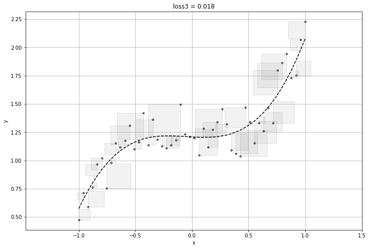
features3 = np.array([[xval**3, xval**2, xval] for xval in x_train])
features4 = np.array([[np.cos(np.pi * xval), np.sin(np.pi * xval)] for xval in x_train])
labels = y_train.reshape(-1,1)
#모델과 손실함수
class MyModel(tf.keras.Model):
def __init__(self, dim = 1, **kwargs):
super().__init__(**kwargs)
self.W = tf.Variable(tf.ones([dim,1]), dtype=tf.float32)
self.b = tf.Variable(tf.ones([1]), dtype=tf.float32)
def call(self, x): #x:데이터 x 좌표 [x y]
return tf.matmul(x,self.W) + self.b
loss = lambda y, yhat: tf.reduce_mean(tf.square(yhat-y))
from helper import generate_batches
for i, features in enumerate([features1, features2, features3, features4],1):
#데이터 섞기
np.random.seed(320)
shuffled_id = np.arange(0,len(x_train))
np.random.shuffle(shuffled_id)
shuffled_x_train = features[shuffled_id]
shuffled_y_train = labels[shuffled_id]
#예측모델과 손실함수
num_features = features.shape[1]
model = MyModel(num_features)
#파라미터 설정 및 수치최적화 알고리즘
MaxEpochs = 15
batch_size = 10
lr = 0.1
optimizer = tf.keras.optimizers.Adam(lr)
#스토캐스틱 방법
for epoch in range(MaxEpochs):
if epoch % 5 == 0 :
curr_loss = loss(labels,model(features))
print(model.W.numpy(), model.b.numpy(), curr_loss.numpy())
for x_batch, y_batch in generate_batches(batch_size, shuffled_x_train, shuffled_y_train):
with tf.GradientTape() as tape:
curr_loss = loss(y_batch,model(x_batch))
gradients = tape.gradient(curr_loss,model.trainable_variables)
optimizer.apply_gradients(zip(gradients,model.trainable_variables))
prediction_values = model(features).numpy()
final_loss = loss(labels, prediction_values)
plt.title("loss{} = {:1.3f}".format(i, final_loss))
visualize_l2(prediction_values.reshape(-1), x_train, labels.reshape(-1))
plt.show()[[1.]] [1.] 0.21256347
[[0.51351786]] [1.2713623] 0.0458722
[[0.44244468]] [1.2667447] 0.04476713
[[1.]
 [1.]] [1.] 0.2260313
[[-0.04760678]
 [ 0.54382205]] [1.2689111] 0.048572093
[[0.17435731]
 [0.46753988]] [1.1939602] 0.043223687
[[1.]
 [1.]
 [1.]] [1.] 0.57014674
[[ 0.43706977]
 [-0.01975712]
 [ 0.19586705]] [1.2126927] 0.030156704
[[0.61056805]
 [0.15909195]
 [0.02455963]] [1.2120951] 0.022248512
[[1.]
 [1.]] [1.] 1.1056408
[[-0.27018577]
 [ 0.03585646]] [1.2154461] 0.13722548
[[-0.01640769]
 [ 0.10837883]] [1.252276] 0.107143074
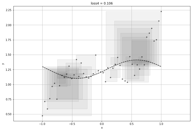
feature를 위와 같이 하나씩 만들어 내어 loss가 가장 작은 함수를 찾으면 되겠지만, 매번 사람이 찾아낼 수는 없기에 우리는 신경망 모델이 필요로 한다.
그럼 다음을 보고 같이 신경망 모델을 만들어 보자.
import numpy as np
import matplotlib.pylab as plt
import tensorflow as tf
plt.rcParams['figure.figsize'] = (12,8)
np.random.seed(327)
x_train = np.linspace(-1,1,50)
y_train = x_train**3 + 0.1 * x_train**2 - 0.15 * x_train + 1.0 + 0.5 * np.random.rand(len(x_train))
features = np.array([[xval] for xval in x_train])
labels = y_train.reshape(-1,1)
class MyModel(tf.keras.Model):
def __init__(self, **kwargs):
super().__init__(**kwargs)
num_hidden1 = 10 #은닉층1의 노드 개수
num_hidden2 = 10 #은닉층2의 노드 개수 #모델의 형태가 달라짐 ->성능도 달라짐
#은닉층 1의 Weight 와 Bias
self.W1 = tf.Variable(tf.random.normal([1, num_hidden1],seed = 624))
self.b1 = tf.Variable(tf.random.normal([num_hidden1],seed = 624))
#은닉층 2의 Weight 와 Bias
self.W2 = tf.Variable(tf.random.normal([num_hidden1, num_hidden2],seed = 624))
self.b2 = tf.Variable(tf.random.normal([num_hidden2],seed = 624))
#출력층의 Weight 와 Bias
self.W3 = tf.Variable(tf.random.normal([num_hidden2, 1],seed = 624))
self.b3 = tf.Variable(tf.random.normal([1],seed = 624))
def call(self,x):
l1 = tf.matmul(x, self.W1) + self.b1 #은닉층 1의 로짓 계산
h1 = tf.nn.sigmoid(l1) #은닉층 1의 활성함수 계산
l2 = tf.matmul(h1, self.W2) + self.b2 #은닉층 2의 로짓 계산
h2 = tf.nn.sigmoid(l2) #은닉층 2의 활성함수 계산
yhat = tf.matmul(h2, self.W3) + self.b3 #출력층에서 모델의 예측값 계산
return yhat
model = MyModel()
#파라미터/최적화 방법/손실 함수 설정
MaxEpochs = 160
batch_size = 10
lr = 0.1
optimizer = tf.keras.optimizers.Adam(lr)
loss = tf.keras.losses.MeanSquaredError()
#데이터 섞기
np.random.seed(320)
shuffled_id = np.arange(0,len(x_train))
np.random.shuffle(shuffled_id)
shuffled_x_train = features[shuffled_id]
shuffled_y_train = labels[shuffled_id]
#모델 컴파일
model.compile(optimizer = optimizer, loss = loss)
#모델 학습
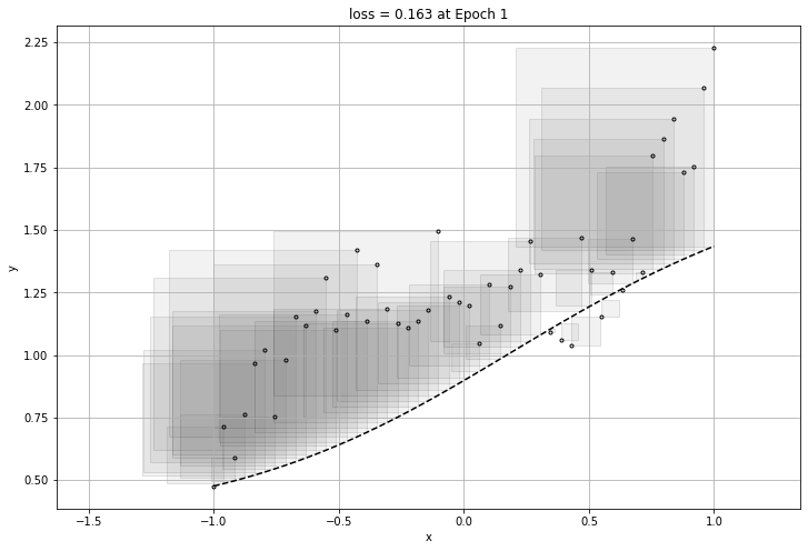
model.fit(shuffled_x_train, shuffled_y_train, epochs = MaxEpochs, batch_size = batch_size, shuffle = False)
prediction_values = model(features).numpy()
final_loss = model.evaluate(features, labels)
plt.title("loss = {:1.3f} at Epoch {}".format(final_loss, MaxEpochs))
visualize_l2(prediction_values.reshape(-1), x_train, labels.reshape(-1))
plt.show()
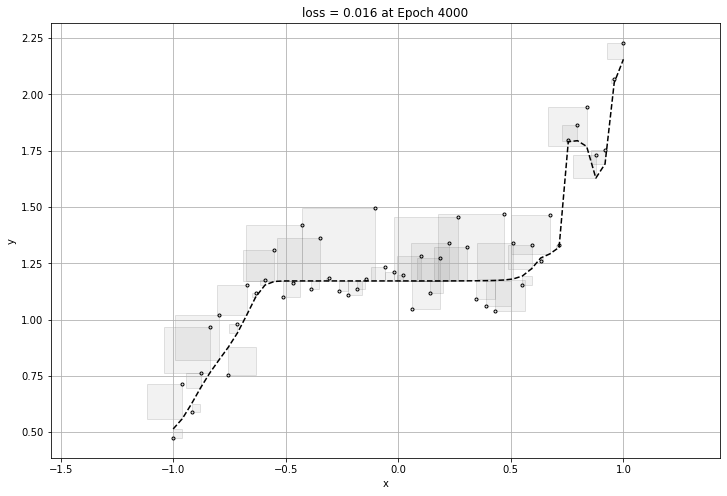
160번의 epochs가 돌아가며 가장 작은 loss를 구할 것이고 구한 loss에 대한 그래프를 뽑아내어 보겠다.
2/2 [==============================] - 0s 3ms/step - loss: 0.0170
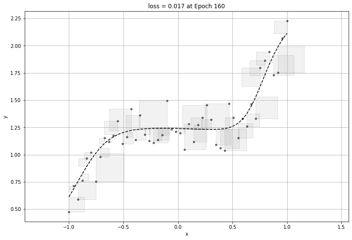
여기까지만 보면 신경망 모델에는 문제가 없이 아주 좋은 성능을 가졌다고 볼 수있다.
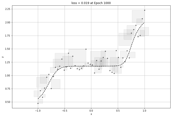
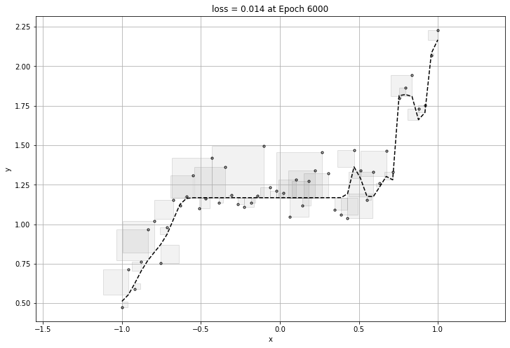
하지만 너무 데이터에 적합하게 만들게 된다면 그 그래프는 일반화가 될 수 없는 그래프이므로, 적당할 때에 epoch이 멈추어야한다.
바로 과적합(overfitting) 문제이다.
아래는 과적합이 된 그래프의 loss와 그래프이다.
0.06322043
0.019019596
0.017578239
0.017660964
0.01769889
0.017711144
0.017718326
0.017800426
0.023232343
0.01868927
0.019399257
0.020247348
0.020244699
0.020963194
0.018823037
0.014845096
0.017425742
0.014041193
0.016706673
0.013994175

0.017518502
0.014298445
0.018744964
0.014099488
0.01430436
0.014203322
0.013823924
0.013224465
0.014069425
0.018034253
0.012950024
0.013585232
0.013528126
0.017079292
0.012679674
0.012655312
0.015305795
0.0128742745
0.012914993
0.012626667
0.016176308
0.013832619
0.012693822
0.01252093
0.0125182895
0.0127047505
0.0132341925
0.012359517
0.012058666
0.012371765
0.013053888
0.015424484
0.012325151
0.011472208
0.011380278
0.013084
0.012158499
0.012902468
0.011846168
0.011938856
0.014138812
0.014132407
0.012726571
0.011635866
0.011529076
0.013155644
0.013579983
0.01253784
0.0129140485
0.015027115
0.013535746
0.012488185
0.014971878
0.014023567
0.013694704
0.012351054
0.012403679
0.011408466
0.0139325475
0.011588365
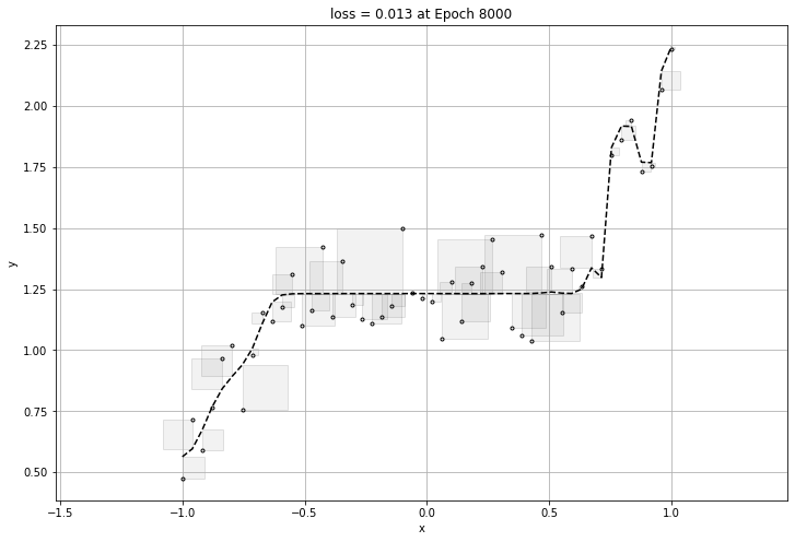
그러므로 overfitting을 방지하기 위해서는 early stop을 걸어주거나, epoch을 줄이는 등의 방법이 있다.
그 와는 반대로 데이터가 너무 적어 underfitting이 되는 경우도 있다. 이 경우에는 데이터를 추가로 더 넣거나, 충분한 데이터가 있음에도 underfitting일 경우에는 epoch을 크게하는 방법 등이 있다.
'Math > Numerical Analysis' 카테고리의 다른 글
| [수치해석] Tensorflow 이용 기본 모델 학습 (0) | 2022.02.11 |
|---|---|
| [수치해석] 수치최적화 알고리즘2 (Adagrad, RMSProp, Adam) (0) | 2022.02.11 |
| [수치해석] 수치최적화 알고리즘(SGD, Momentum) (0) | 2022.02.11 |